PyTorch 是什么?
基于 Python 的科学计算包,服务于以下两种场景:
- Numpy 的替代品,可以使用 GPU 的强大计算力
- 提供最大的灵活性和高速的深度学习研究平台
Tensors
Tensors 与 Numpy 中的 ndarrays 类似,但是在 PyTorch 中 Tensors 可以使用 GPU 进行计算。
1
2
| from __future__ import print_function
import torch
|
[ 1 ] 创建一个 5x3 的矩阵,但不初始化:
1
2
3
4
5
6
7
| x = torch.empty(5, 3)
print(x)
# tensor([[0.0000, 0.0000, 0.0000],
# [0.0000, 0.0000, 0.0000],
# [0.0000, 0.0000, 0.0000],
# [0.0000, 0.0000, 0.0000],
# [0.0000, 0.0000, 0.0000]])
|
[ 2 ] 创建一个随机初始化的矩:
1
2
3
4
5
6
7
| x = torch.rand(5, 3)
print(x)
# tensor([[0.6972, 0.0231, 0.3087],
# [0.2083, 0.6141, 0.6896],
# [0.7228, 0.9715, 0.5304],
# [0.7727, 0.1621, 0.9777],
# [0.6526, 0.6170, 0.2605]])
|
[ 3 ] 创建一个 0 填充的矩阵,数据类型为 long:
1
2
3
4
5
6
7
| x = torch.zero(5, 3, dtype=torch.long)
print(x)
# tensor([[0, 0, 0],
# [0, 0, 0],
# [0, 0, 0],
# [0, 0, 0],
# [0, 0, 0]])
|
[ 4 ] 创建一个 tensor 使用现有数据初始化:
1
2
3
4
5
| x = torch.tensor(
[5.5, 3]
)
print(x)
# tensor([5.5000, 3.0000])
|
[ 5 ] 根据现有的 tensor 创建 tensor。这些方法将重用输入 tensor 的属性(如:dtype,除非设置新的值进行覆盖):
 1
 2
 3
 4
 5
 6
 7
 8
 9
10
11
12
13
14
15
16
17
| # 利用 new_* 方法创建对象
x = x.new_ones(5, 3, dtype=torch.double)
print(x)
# tensor([[1., 1., 1.],
# [1., 1., 1.],
# [1., 1., 1.],
# [1., 1., 1.],
# [1., 1., 1.]], dtype=torch.float64)
# 覆盖 dtype
# 对象 size 相同,只是 值和类型 发生变化
print(x)
# tensor([[ 0.5691, -2.0126, -0.4064],
# [-0.0863, 0.4692, -1.1209],
# [-1.1177, -0.5764, -0.5363],
# [-0.4390, 0.6688, 0.0889],
# [ 1.3334, -1.1600, 1.8457]])
|
[ 6 ] 获取 size:
1
2
| print(x.size())
# torch.Size([5, 3])
|
Tip:
torch.Size 返回 tuple 类型,支持 tuple 类型所有的操作。
[ 7 ] 操作
[ 7.1 ] 加法:
 1
 2
 3
 4
 5
 6
 7
 8
 9
10
11
12
13
14
| y = torch.rand(5, 3)
print(x+y)
# tensor([[ 0.7808, -1.4388, 0.3151],
# [-0.0076, 1.0716, -0.8465],
# [-0.8175, 0.3625, -0.2005],
# [ 0.2435, 0.8512, 0.7142],
# [ 1.4737, -0.8545, 2.4833]])
print(torch.add(x, y))
# tensor([[ 0.7808, -1.4388, 0.3151],
# [-0.0076, 1.0716, -0.8465],
# [-0.8175, 0.3625, -0.2005],
# [ 0.2435, 0.8512, 0.7142],
# [ 1.4737, -0.8545, 2.4833]])
|
提供输出 tensor 作为参数:
1
2
3
4
5
6
7
8
| result = torch.empty(5, 3)
torch.add(x, y, out=result)
print(result)
# tensor([[ 0.7808, -1.4388, 0.3151],
# [-0.0076, 1.0716, -0.8465],
# [-0.8175, 0.3625, -0.2005],
# [ 0.2435, 0.8512, 0.7142],
# [ 1.4737, -0.8545, 2.4833]])
|
[ 7.2 ] 替换:
1
2
3
4
5
6
7
8
| # add x to y
y.add_(x)
print(y)
# tensor([[ 0.7808, -1.4388, 0.3151],
# [-0.0076, 1.0716, -0.8465],
# [-0.8175, 0.3625, -0.2005],
# [ 0.2435, 0.8512, 0.7142],
# [ 1.4737, -0.8545, 2.4833]])
|
{% note info %}
_ 结尾的操作会替换原变量。
如:x_copy_(y),x.t_() 会改变 x
{% endnote %}
[ 7.3 ] 使用 Numpy 中索引方式,对 tensor 进行操作:
1
2
| print(x[:, 1])
# tensor([-2.0126, 0.4692, -0.5764, 0.6688, -1.1600])
|
[ 8 ] torch.view 改变 tensor 的维度和大小 (与 Numpy 中 reshape 类似):
1
2
3
4
5
6
| x = torch.randn(4, 4)
y = x.view(16)
z = x.view(-1, 8) # -1 从其他维度推断
print(x.size(), y.size(), z.size())
# torch.Size([4, 4]) torch.Size([16]) torch.Size([2, 8])
|
[ 9 ] 如果只有一个元素的 tensor,使用 item() 获取 Python 数据类型的数值:
1
2
3
4
5
| x = torch.randn(1)
print(x)
print(x.item())
# tensor([-0.2368])
# -0.23680149018764496
|
Numpy 转换
Torch Tensor 与 Numpy 数组之间进行转换非常轻松。
1
2
3
4
5
| a = torch.ones(5)
b = a.numpy()
print(a) # tensor([1., 1., 1., 1., 1.])
print(b) # [1. 1. 1. 1. 1.]
|
Torch Tensor 与 Numpy 数组共享底层内存地址,修改一个会导致另一个的变化。
1
2
3
4
| a.add_(1)
print(a) # tensor([2., 2., 2., 2., 2.])
print(b) # [2. 2. 2. 2. 2.]
|
1
2
3
4
5
6
7
| import numpy as np
a = np.ones(5)
b = torch.from_numpy(a)
np.add(a, 1, out=a)
print(a) # [2. 2. 2. 2. 2.]
print(b) # tensor([2., 2., 2., 2., 2.], dtype=torch.float64)
|
Tip:
所有的 Tensor 类型默认都是基于 CPU, CharTensor 类型不支持到 Numpy 的装换。
CUDA 张量
使用 .to() 可以将 Tensor 移动到任何设备中。
1
2
3
4
5
6
7
| if torch.cuda.is_available():
device = torch.device('cuda') # CUDA 设备对象
y = torch.ones_like(x, device=device) # 直接从 GPU 创建张量
x = x.to(device)
z = x + y
print(z) # tensor([0.7632], device='cuda:0')
print(z.to('cpu', torch.double)) # tensor([0.7632], dtype=torch.float64)
|
Autograd 自动求导
autograd 包为 Tensor 上所有的操作提供了自动求导。它是一个运行时定义的框架,这意味着反向传播是根据你的代码来确定如何运行,并且每次迭代可以是不同的。
正向传播 反向传播
神经网络(NN)是在某些输入数据上执行嵌套函数的集合。
这些函数由参数(权重和偏差组成)定义,参数在 PyTorch 中存储在张量中。
训练 NN 分为两个步骤:
- 正向传播:在正向传播中,NN 对正确的输出进行最佳猜测。它通过每个函数运行输入数据以进行猜测。
- 反向传播:在反向传播中,NN 根据其猜测中的误差调整其参数。它通过从输出向后遍历,收集有关参数(梯度)的误差导数并使用梯度下降来优化参数来实现。
[ 1 ] 我们从 torchvision 加载了经过预训练的 resnet18 模型。创建一个随机数据张量来表示具有 3 个通道的单个图像,高度和宽度为 64,其对应的label初始化为一些随机值。
1
2
3
4
5
| import torch, torchvision
model = torchvision.models.resnet18(pretrained=True)
data = torch.rand(1, 3, 64, 64)
labels = torch.rand(1, 1000)
|
[ 2 ] 接下来,通过模型的每一层运行输入数据进行预测。正向传播。
1
| prediction = model(data)
|
[ 3 ] 使用模型的预测(predication)和相应的标签(labels)来计算误差(loss)。
下一步通过反向传播此误差。我们在 loss tensor 上调用 .backward() 时,开始反向传播。Autograd 会为每个模型参数计算梯度并将其存储在参数 .grad 属性中。
1
2
| loss = (prediction - labels).sum()
loss.backword() # backword pass
|
[ 4 ] 接下来,我们加载一个优化器(SDG),学习率为 0.01,动量为 0.9。在 optim 中注册模型的所有参数。
1
| optim = torch.optim.SDG(model.parameters(), lr=1e-2, momentum=0.9)
|
[ 5 ] 最后,调用 .step() 启动梯度下降。优化器通过 .grad 中存储的梯度来调整每个参数。
1
| optim.step() # gradient descent
|
神经网络的微分
这一小节,我们将看看 autograd 如何收集梯度。
我们在创建 Tensor 时,使用 requires_grad=True 参数,表示将跟踪 Tensor 的所有操作。
1
2
3
4
5
6
7
| import torch
a = torch.tensor([2., 3.], require_grad=True)
b = torch.tensor([6., 4.], require_grad=True)
# 从 tensor a, b 创建另一个 tensor Q
Q = 3*a**3 - b**2
|
假设 tensor a,b 是神经网络的参数,tensor Q 是误差。在 NN 训练中,我们想要获得相对于参数的误差,即各自对应的偏导:
$$\frac{\partial Q}{\partial a}=9a^2$$
当我们在 tensor Q 上调用 .backward() 时,Autograd 将计算这些梯度并将其存储在各个张量的 .grad 属性中。
我们需要在 Q.backword() 中显式传递 gradient 参数(与 Q 形状相同的张量,表示 Q 相对本身的梯度)。
$$\frac{\partial Q}{\partial b}=-2b$$
1
2
3
4
5
6
7
8
| external_grad = torch.tensor([1., 1.])
Q.backward(gradient=external_grad)
# 最后,梯度记录在 a.grad b.grad 中,查看收集的梯度是否正确
print(9*a**2 == a.grad)
# tensor([True, True])
print(-2*b == b.grad)
# tensor([True, True])
|
我们也可以将 Q 聚合为一个标量,然后隐式地向后调用,如:Q.sum().backward()。
神经网络
上一节,我们了解到 nn 包依赖 autograd 包来定义模型并求导。下面,我们将了解如何定义一个网络。一个 nn.Module 包含个 layer 和一个 forward(input) 方法,该方法返回 output。
如下,这是一个对手写数字图像进行分类的卷积神经网络:
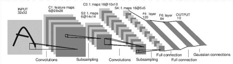
神经网络的典型训练过程如下:
- 定义包含一些可学习的参数(权重)神经网络模型
- 在数据集上迭代
- 通过神经网络处理输入
- 计算损失(输出结果和正确值的差值大小)
- 将梯度反向传播回网络的参数
- 更新网络的参数(梯度下降):weight = weight - learning_rate * gradient
定义网络
在模型中必须定义 forward(), backword(用来计算梯度)会被 autograd 自动创建。可在 forward() 中使用任何针对 Tensor 的操作。
 1
 2
 3
 4
 5
 6
 7
 8
 9
10
11
12
13
14
15
16
17
18
19
20
21
22
23
24
25
26
27
28
29
30
31
32
33
34
35
36
37
38
39
40
41
42
43
44
45
| import torch
import torch.nn as nn
import torch.nn.functional as F
class Net(nn.Model):
def __init__(self):
super(Net, self).__init__()
# 1 input image channel, 6 output channels, 3x3 square convolution
# kernel
self.conv_1 = nn.Conv2d(1, 6, 3)
self.conv_2 = nn.Conv2d(6, 16, 3)
# an affine operation: y = Wx + b
self.fc1 = nn.Linear(16 * 6 *6, 120)
self.fc2 = nn.Linear(120, 84)
self.fc3 = nn.Linear(84, 10)
def forward(self, x):
# Max Pooling over a (2, 2) window
x = F.max_pool2d(F.relu(self.conv1(x)), (2, 2))
# If the size is a square you can only specify a single number
x = F.max_pool2d(F.relu(self.conv2(x)), 2)
x = x.view(-1, self.num_flat_features(x))
x = F.relu(self.fc1(x))
x = F.relu(self.fc2(x))
x = self.fc3(x)
return x
def num_flat_features(sefl, x):
size = x.size()[1: ] # all dimensions except the batch dimension
num_features = 1
for s in size:
num_features *= s
return num_features
net = Net()
print(net)
# Net(
# (conv1): Conv2d(1, 6, kernel_size=(3, 3), stride=(1, 1))
# (conv2): Conv2d(6, 16, kernel_size=(3, 3), stride=(1, 1))
# (fc1): Linear(in_features=576, out_features=120, bias=True)
# (fc2): Linear(in_features=120, out_features=84, bias=True)
# (fc3): Linear(in_features=84, out_features=10, bias=True)
# )
|
parameters() 返回可被学习的参数(权重)列表和值
1
2
3
4
| params = list(net.parameters())
print(len(params)) # 10
print(params[0].size()) # conv1 的 weight torch.Size([6, 1, 3, 3])
|
测试随机输入 32x32。注:这个网络(LeNet)的期望的输入大小是 32x32,如果使用 MINIST 数据集来训练这个网络,请把图片大小重新调整到 32x32。
1
2
3
4
5
| input = torch.randn(1, 1, 32, 32)
out = net(input)
print(out)
# tensor([[ 0.1120, 0.0713, 0.1014, -0.0696, -0.1210, 0.0084, -0.0206, 0.1366,
# -0.0455, -0.0036]], grad_fn=<AddmmBackward>)
|
将所有的参数的梯度缓存清零,进行随机梯度的反向传播。
1
2
| net.zero_grad()
out.backward(torch.randn(1, 10))
|
Tip:
torch.nn 仅支持小批量输入。整个 torch.nn 包都只支持小批量样本,而不支持单个样本。
如:nn.Conv2d接受一个4维 Tensor,分别维 sSamples * nChannels * Height * Width (样本数* 通道数 * 高 * 宽)。如果你有单个样本,只需要使用 input.unsqueeze(0) 来添加其他的维数。
至此,我们大致了解了如何构建一个网络,回顾一下到目前为止使用到的类。
torch.Tensor: 一个多维数组。 支持使用 backward() 进行自动梯度计算,并保存关于这个向量的梯度 w.r.t.
nn.Model: 神经网络模块。实现封装参数、移动到 GPU 上运行、导出、加载等。
nn.Parameter: 一种张量。将其分配为 Model 的属性时,自动注册为参数。
autograd.Function: 实现一个自动求导操作的前向和反向定义。每个 Tensor 操作都会创建至少一个 Function 节点,该节点连接到创建 Tensor 的函数,并编码其历史记录。
损失函数
1
2
3
4
5
6
7
8
9
| output = net(input)
target = torch.randn(10) # 例子:一个假设的结果
target = target.view(1, -1) # 让 target 与 output 的形状相同
criterion = nn.MSELoss()
loss = criterion(output, target)
print(loss)
|
反向传播
要实现反向传播误差,只需要 loss.backward()。
但是,需要清除现有的梯度,否则梯度将累积到现有的梯度中。
1
2
3
4
5
6
7
| net.zero_grad() # 将所有的梯度缓冲归零
print(net.conv1.bias.grad) # conv1.bias.grad 反向传播前 tensor([0., 0., 0., 0., 0., 0.])
loss.backward()
print(net.conv1.bias.grad) # 反向传播后 tensor([0.0111, -0.0064, 0.0053, -0.0047, 0.0026, -0.0153])
|
更新权重
在使用 PyTorch 时,可以使用 torch.optim 中提供的方法进行梯度下降。如:SDG,Nesterov-SDG,Adam,RMSprop 等。
 1
 2
 3
 4
 5
 6
 7
 8
 9
10
11
| import torch.optim as optim
# 创建一个 optimizer
optimizer = optim.SDG(net.parameters(), lr=0.01)
# 在训练中循环
optimizer.zero_grad() # 将梯度缓冲区清零
output = net(input)
loss = criterion(output, target)
loass.backword()
optimizer.step() # 更新
|
训练分类器
数据从哪里来?
通常,需要处理图像、文本、音频或视频数据时,可以使用将数据加载到 NumPy 数组中的标准 Python 包,再将该数值转换为 torch.*Tensor。
- 处理图像,可以使用 Pillow,OpenCV
- 处理音频,可以使用 SciPy,librosa
- 处理文本,可基于 Python 或 Cython 的原始加载,或 NLTK 和 SpaCy
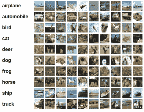
对于图像任务,其中包含了一个 torchvision 的包,含有常见的数据集(Imagenet,CIFAR10,MNIST等)的数据加载器,以及用于图像的数据转换器(torchvision.datasets 和 torch.utils.data.DataLoader)。
在本示例中,将使用 CIFAR10 数据集。其中包含 10 分类的图像:“飞机”,“汽车”,“鸟”,“猫”,“鹿”,“狗”,“青蛙”,“马”,“船”,“卡车”。图像的尺寸为 3 * 32 * 32,即尺寸为 32 * 32 像素的 3 通道彩色图像。
接下来,作为演示,将按顺序执行以下步骤训练图像分类器:
- 使用
torchvision 加载并标准化 CIFAR10 训练和测试数据集 - 定义 CNN
- 定义损失函数
- 根据训练数据训练网络
- 在测试数据上测试网络
加载并标准化 CIFAR10
1
2
3
| import torch
import torchvision
import torchvision.transforms as transforms
|
torchvision 的输出是 [0, 1] 的 PILImage 图像,我们要把它转换为归一化范围为 [-1, 1] 的张量。
 1
 2
 3
 4
 5
 6
 7
 8
 9
10
11
| transform = transforms.Compose(
[transforms.ToTensor(), transforms.Normalize((0.5, 0.5, 0.5), (0.5, 0.5, 0.5))]
)
trainset = torchvision.datasets.CIFAR10(root='./data', train=True, download=True, transform=transform)
trainloader = torch.utils.data.DataLoader(trainset, batch_size=4, shuffle=True, num_workers=2)
testset = trochvision.datasets.CIFAR10(root='./data', train=False, download=True, transform=transform)
testloader = torch.utils.data.DataLoader(testset, barch_size=4, shuffle=False, num_workers=2)
classes = ('plane', 'car', 'bird', 'cat', 'deer', 'dog', 'frog', 'horse', 'ship', 'truck')
|
定义 CNN
 1
 2
 3
 4
 5
 6
 7
 8
 9
10
11
12
13
14
15
16
17
18
19
20
21
22
23
24
25
26
27
28
| import torch.nn as nn
import torch.nn.functional as F
class Net(nn.Module):
def __init__(self):
super(Net, self).__init__()
# in_channels, out_channels, kernel_size
# 输入的为 3 通道图像,提取 6 个特征,得到 6 个 feature map,卷积核为一个 5*5 的矩阵
self.conv1 = nn.Conv2d(3, 6, 5)
self.pool = nn.MaxPool2d(2, 2)
self.conv2 = nn.Conv2d(6, 16, 5)
# 卷积层输出了 16 个 feature map,每个 feature map 是 6*6 的二维数据
self.fc1 = nn.Linear(16 * 5 * 5, 120)
self.fc2 = nn.Linear(120, 84)
self.fc3(84, 10)
def forward(self, x):
x = self.pool(F.relu(self.conv1(x)))
x = self.pool(F.relu(self.conv2(x)))
x = x.view(-1, 16 * 5 * 5)
x = F.relu(self.fc1(x))
x = F.relu(self.fc2(x))
x = self.fc3(x)
return x
net = Net(s)
|
定义损失函数和优化器
这里我们使用交叉熵作为损失函数,使用带动量的随机梯度下降。
1
2
3
4
| import torch.optim as optim
criterion = nn.CrossEntropyLoss()
optimizer = optim.SDG(net.parameters(), lr=0.001, momentum=0.9)
|
训练网络
接下来,只需要在迭代数据,将数据输入网络中并优化。
 1
 2
 3
 4
 5
 6
 7
 8
 9
10
11
12
13
14
15
16
17
| for epoch in range(2):
running_loss = 0.0
for i, data in enumerate(trainloader, 0):
inputs, labels = data # 获取输入
optimizer.zero_grad() # 将梯度缓冲区清零
outputs = net(inputs) # 正向传播
loss = criterion(outputs, lables)
loss.backward() # 反向传播
optimizer.step() # 优化
running_loss += loss.item()
if i % 2000 == 1999: # 每 2000 批次打印一次
print('[]' % (epoch+1, i+1, running_loss / 2000))
running_loss = 0.0
|
在测试集上测试数据
在上面的训练中,我们训练了 2 次,接下来,我们要检测网络是否从数据集中学习到了有用的东西。通过预测神经网络输出的类别标签与实际情况标签对比进行检测。
 1
 2
 3
 4
 5
 6
 7
 8
 9
10
11
12
| corrent = 0
total = 0
with torch.no_grad():
for data in testloader:
images, lobels = data
outputs = net(images)
_, predicted = torch.max(outputs.data, 1)
total += labels.size(0)
corrent += (predicted == labels).sum().item()
print('Accuracy of the network on the 10000 test images: %d %%' % (100 *corrent / total))
# Accuracy of the network on the 10000 test images: 9%
|
在训练两次的网络中,随机选择的正确率为 10%。网络似乎学到了一些东西。
那这个网络,识别哪一类好,哪一类不好呢?
 1
 2
 3
 4
 5
 6
 7
 8
 9
10
11
12
13
14
15
16
17
18
19
20
21
22
23
24
25
26
27
28
| class_corrent = list(0. for i in range(10))
class_total = list(0. for i in range(10))
with torch.no_grad():
for data in testloader:
images, labels = data
outputs = net(images)
_, predicted = torch.max(outputs, 1)
c = (predicted == labels).squeeze()
for i in range(4):
label = labels[i]
class_correct[label] += c[i].item()
class_total[label] += 1
for i in range(10):
print('Accuracy of %5s : %2d %%' % (classes[i], 100 * class_correct[i] / class_total[i]))
# Accuracy of plane : 99 %
# Accuracy of car : 0 %
# Accuracy of bird : 0 %
# Accuracy of cat : 0 %
# Accuracy of deer : 0 %
# Accuracy of dog : 0 %
# Accuracy of frog : 0 %
# Accuracy of horse : 0 %
# Accuracy of ship : 0 %
# Accuracy of truck : 0 %
|
使用 GPU
与将 tensor 移到 GPU 上一样,神经网络也可以移动到 GPU 上。
如果可以使用 CUDA,将设备定义为第一个 cuda 设备:
1
2
3
4
| device = torch.device('cuda:0' if torch.cuda.is_available() else 'cpu')
print(device)
# cuda:0
|
复制 nn 和 tensor 到 GPU 上。
1
2
3
| model = net.to(device)
inputs, labels = data[0].to(device), data[1].to(device)
|
Tip:
使用 .to(device) 并没有复制 nn / tensor 到 GPU 上,而是返回了一个 copy。需要赋值到一个新的变量后在 GPU 上使用这个 nn / tensor。
参考